Running IBM PC APL in DOSBox

This blog post is going to be really short. After I’ve published my last post about IBM Personal Computer APL version 1.00 a friend of mine asked me for help with running APL in DOSBox. In general I try to avoid working with PC emulators and I really try to avoid working with DOSBox. Especially on macOS. So, I downloaded DOSBox and run APL.EXE just to get the following error.

Fortunately, it turned out that CodeView debugger works like a charm in DOSBox so I was able to find out why APL crashes. In short, APL doesn’t compare correctly the available system memory. The fix is simple. Before you start, make sure that your APL.EXE has the following SHA1 553043de3cec8a05605838d23dd9de7c129bc80e. If this is not case then don’t apply the fix.

Here is the patch as a text (not sure if DOSBox supports copy/paste).


ren apl.exe apl.bin
debug apl.bin
-e 47A
xxxx:047A     7D. 73
-w
-q
ren apl.bin apl.exe
apl.exe

The newly patched APL.EXE now should have the following SHA1 cc0d16dafd2309117d8b758ecc90a0c6f7e7a313. After applying the above patch you should be able run APL.EXE in DOSBox.

Hope this helps.

Those were the days – part 5

In this post I am going to share my experience with IBM Personal C0mputer APL version 1.00. As with the previous posts from this blog post series I am not going into the details of the language itself, but rather share my first impressions from working with APL and try to extrapolate what might be working professionally with it back in 1983.

According the documentation it was released in May 1983. This makes it the first programming language IBM released after PC-DOS 2.00 which was released in March 1983. The first thing that caught my eye was the documentation cover title “APL by IBM Madrid Scientific Center”. This resonated with the only two facts I knew about APL – it was created by Kenneth Iverson who is ACM Turing Award laureate and the language reputation for heavily using mathematical notation. So far, the programming languages I previously covered in this blog post series were implemented by Microsoft, so I was curious to see what IBM implemented for IBM PC.

My work setup is same as before – a Bulgarian clone of IBM PC with 256KB, math coprocessor, CGA monitor and two 360KB floppy drives. Also, my learning approach was same as before – I mostly relied on reading the official IBM documentation, and when necessary time correct books from early 1980s. So, I started reading the documentation. Just after a couple of pages I read the requirement for 8087 coprocessor. On one hand, this was a pleasant surprise considering my experience with IBM Fortran Compiler 1.00/2.00. On the other hand, Intel 8087 coprocessor was quite expensive in the early 1980s so IBM PC APL was meant as a niche product. On the software side IBM PC APL version 1.00 requires PC-DOS 2.00 which supports 360KB floppies and thus made my life much easier as working with old floppy disks on old hardware could be nerve-wracking.

As I said, I had no previous knowledge about APL so I was surprised to see what happened when I run APL.EXE

NOTE: As usual I am going to use screenshots from a PC emulator rather than taking poor quality pictures with my mobile phone. My initial intention was to use Marty PC emulator as it helped me a lot in my previous projects. However, at the time of writing, it has no official support for 8087. After I a quick internet search I’ve found 86Box project which I am going to use for making screeenshots for this post.

One of the perks of working with actual hardware, and in my case with quite old hardware, is that you constantly get audio and video feedback. A few seconds after I run APL.EXE I heard the familiar “click” sound when my old CGA monitor changes video mode and I saw what definitely is graphics mode. It didn’t surprised me because, as I said, I knew about the language reputation for using mathematical notation, and it makes sense use graphics mode to render mathematical symbols. Frankly, I find it a bold move considering how many years later PC-DOS 5.00 would be the first DOS supporting *.CPI files and custom code pages. Many other software developers would bend the language specification/requirements and implement plain text environment. In the case of APL it only shows how much important is the visual use of mathematical notation.

Now, I have to discuss somewhat controversial topic. APL is designed to be used with custom keyboard layout. This was well documented and IBM even provided nice keyboard drawings to make the learning process easier. So, I had to print the documentation and look at drawings whenever I was not sure where a symbol is located.

I am not going to discuss key overstriking, but I can relate to the people who are complaining about it. It took me a few days to become semi-fluent in typing APL programs. What I find fascinating is that even today’s modern APL implementations follow the same input methods as in 1980s (to be fair, they also support more ergonomic input methods).

Having put this issue aside, APL also use unpopular way to parse expressions. While there is nothing inherently wrong with it, there are good reasons why we use the current standardized way to define precedence. In short (and somewhat oversimplified), APL has no order of operations and expressions are evaluated right to left. As I said, there is nothing wrong per se, but this could surprise a lot of people in the beginning.

I have to say that I had to be focused when I was typing math expressions and maybe I used parenthesis a little too much, but better safe than sorry.

Before I discuss the APL work environment, I am going to share my thoughts on the idea of using work environment when it comes to programming languages. I fully appreciate using work environment in specialized software like CAD/CAM, computing systems like Mathematica and Maple, or even game development software like Unity, but I don’t think it is a good idea to have specialized work environment for a programming language. Logo is an exception rather than a rule. Work environments for programming languages can be a great thing for educational purposes, but not when they are used professionally. We solved the problem of standardization of execution of the programs we write, by standardizing the interpreters, compilers, runtimes/virtual machines, and even docker/kubernetes if you will. I do understand the mainframe legacy of APL, for example in IBM/360, but when you design a product for personal computers, as in the name of IBM PC, you must adapt to new the requirements. That being said, the APL work environment offers the concept of workspace (*.AIO files). This makes it relatively easy to organize and/or migrate code.

After I’ve got basic knowledge about APL and its environment, it was time to decide what I should implement. As with COBOL, I had a hard time deciding what to implement. APL is often regarded as an excellent language for array processing, especially when mathematical operations are heavily involved. The hardware requirement for math coprocessor also suggests this. I don’t know whether APL uses row-major order and column-major order, so I decided to implement a program that calculates matrix determinant and check it in practice. I’ve decided to go with the classic Gaussian elimination algorithm (mostly naive implementation).


 R←CALCDET A;M;N;I;J;K;T;P
 M←A
 N←1↑⍴M
 P←1
 I←1
L1:→(I>N)/L7
 K ←I
 J←I
L2:J←J+1
 →(J>N)/L3
 →((|M[J;I])≤|M[K;I])/L2
 K←J
 →L2
L3:→(K=I)/L4
 T←M[I;]
 M[I;]←M[K;]
 M[K;]←T
 P←-P
L4:→(M[I;I]=0)/L8
 J←I
L5:J←J+1
 →(J>N)/L6
 M[J;]←M[J;]-(M[J;I]÷M[I;I])×M[I;]
 →L5
L6:I←I+1
 →L1
L7:R←P××/1 1⍉M
 →0
L8:R←0

Not knowing much about APL, I was satisfied with the program. That was until I was reading the documentation how to do more advanced function printing and/or editing when I saw that IBM had also provided an example program that calculates matrix determinant.

 Z←DET A;B;P;I
 I←⌷IO
 Z←1
L:P←(|A[;I])⍳⌈/|A[;I]
 →(P=I)/LL
 A[I,P;]←A[P,I;]
 Z←-Z
LL:Z←Z×B←A[I;I]
 →(0 1∨.=Z,1↑⍴A)/0
 A←1 1↓A-(A[;I]÷B)∘.×A[I;]
 →L

I saw that IBM implementation is much faster than mine so I started to analyze the function. While their implementation is not hard to grasp (tricks like A[I,P;]←A[P,I;] are nice, but are just tricks) I realized that I probably won’t easily come with the idea for this concrete implementation.

This provoked me to think. At first glance both implementations use the same Gaussian elimination algorithm. Yet, one is much more efficient than the other. Think about the following oversimplified example. You can do multiplication by doing addition over and over again, or use the traits of positional number system. In both cases the end result will be the same, but the former is much less efficient than the latter. A programmer can easily detect and understand explicit loops. However, the problem becomes much less explicit when a chain of function composition is involved. To solve this kind of problems you must have deep knowledge of the programming language and its libraries or built-in functions. This problem is not unique to APL, but so far I haven’t seen another language where it is so noticeable.

All this was a bit disheartening, so I needed a revenge. The way APL documentation is organized is a bit strange. Right after the introduction chapters, the documentation explains what APL auxiliary processors are and how to implement ones. In short, auxiliary processors are a way to escape the work environment and communicate with the operating system and/or hardware. So, I decided to implement an auxiliary processor that calculates matrix determinant using 8087 coprocessor. This time I decided to use Bareiss algorithm. Due to the technical limitations of auxiliary processors I had to constrain the matix elements to integers in the range -32768 to 32767. Not a fair play, but it was all about revenge. The actual implementation is a bit naive and not well optimized, but I was currious how well the built-in APL functions utilize the math coprocessor. My expectation was that my implementation will be on par with IBM implementation.

PERF measures the implementation provided by IBM, PERF2 measures my implementation in APL, and PERF3 measures my implementation in 8087 assembly. As someone who wrote professionally for few years performance and memory profilers I have to make the disclaimer that I also measure the time for ⌷PK to access 0040:006C and that the DOS timer frequency is 18.2065 Hz which for this particular scenario is good enough. Using ⌷PK provided much more stable times than using ⌷AI. Interestingly, the actual values on my IBM PC clone are slightly higher, which only shows that while 86Box is faster, it is a quite precise emulator. Having said that, I was very surprised. As I said, my Bareiss implementation is a bit naive and there is a lot of room for optimizations. Still, it is almost 9 times faster. This is a sure sign that APL uses 8087 sporadically, probably for some very narrow scenarios, like sine/cosine (using ○ circular function) or logarithm (using ⍟ function). You can find the source code and floppy disk image here.

In conclusion, I think IBM Personal Computer APL version 1.00 was good enough product for its time. My main concern is that writing performant APL is harder compared to other languages I know. In hindsight the requirement for custom keyboard layout also didn’t help APL to become more popular. Having said that, APL is a niche language, but still used in some financial organizations. While there are reports that it is still used for data analysis and scientific computing, my research shows that it is extremely rare.

Those were the days – part 4

In this post we will take a look at IBM Personal Computer COBOL version 1.00. It was released in March 1982 and was written by Microsoft. Unlike the previous languages from this blog post series, I knew nothing about COBOL until a month ago. I still don’t know much about it, but so far learning and working with it has been a pleasant experience. As with the previous posts, this post is not going to be about COBOL but rather about my experience with it and things it provoked me to think about.

There are many ways to learn a programming language. Usually, I start with the official language documentation and quickly move to online tutorials. This time I decided to combine reading of the official IBM documentation with two era-correct books “COBOL for the IBM PC” by Pacifico A. Lim and “Programming the IBM Personal Computer: COBOL” by Neill Graham. I spent the last few weeks writing around 50 programs, and I’ve started to get a feeling of what idiosyncratic COBOL looks like. I know there is a bad wrap around COBOL, but as I said, I enjoyed it. It made me curious to learn more about it and this rarely happens when I work with today’s frameworks and languages. Nevertheless, working with a language that has more than 300 keywords can be challenging. This might be the reason why Edsger Dijkstra had a negative view about COBOL. On the other hand, organizations like Gartner provided reports in 2010s claiming there are 100-200 billion lines of COBOL in production. If true, this begs the question of whether COBOL is a “bad” language. So far it seems that COBOL is suitable for enterprise business applications. Considering the fact that the latest COBOL standard is from 2023 I don’t consider it a dead language.

I have to say that I had a difficult time deciding what program to write for this post. COBOL is often said to excel in batch processing, transaction processing, and reporting. As I said, I wrote around 50 programs, some of which were over 2000 lines of code. At the end, I decided to write a short COBOL batch processing program and some MASM code for CGA graphics reporting.

I follow the same floppy disks organization as the one for IBM PC Pascal 1.00 and IBM PC Fortran 1.00.

  • Disk 1 (bare minimum PC DOS 1.00)
    • COBOL.COM
    • COBOL1.OVR
    • COBOL2.OVR
    • COBOL3.OVR
    • COBOL4.OVR
    • EDLIN.COM
  • Disk 2
    • COBOL1.LIB
    • COBOL2.LIB
    • COBRUN.EXE
    • COMMAND.COM
    • LINK.EXE
  • Disk 3 (IBM PC MASM 1.00)
  • Disk 4

I guess I was lucky to try IBM PC COBOL right after IBM PC FORTRAN as both languages follow fixed program format.

As with the previous projects, I used EDLIN and I can say it is good enough for high level language as COBOL. It’s kind of funny but working on a physical CRT monitor helped me develop a “visual” sense where 72nd column is.

A few words about the compiler. It is slow. The error messages are good enough to give you a clue what is wrong. The program’s organization of divisions, sections, paragraphs, sentences, and statements helped a lot, and there were not many compiler errors.

The program reads DATA.TXT file, groups the data, and presents the result as text and graphical reports.

You can edit the data to generate different reports.

While I was preparing the disk images just before publishing this post, I decided to test them in MartyPC emulator. To my surprise, while DISPLAY was working correctly on my Pravetz 16 with VDC-3 CGA video card, a Bulgarian clone of Juko G7, it was printing gibberish on MartyPC emulator. For that reason, I had to implement PRTSTR (print string) functionality in MASM. I hope this implementation will work correctly on other CGA cards.

Another potential problem would be running the program on a PC with 640KB RAM or environments like DOSBox. I touched on this problem in the first blog post of this series. Here is a workaround for this problem.

debug cobol2.lib
-s 0 fff c3 7d 15
xxxx:0920
-e 921
xxxx:0921 7D.7E <===== enter 7E
-w
-q

This will change specific jump instruction from JGE to JLE. Keep in mind that using this patch will prevent running COBOL programs on a PC with less memory.

In case you want to make your compiling and linking experience better on a hard disk drive, you may want to change some "A:" hard coded file paths.

Having said all that, you may wonder what the point of existing IBM PC COBOL is, and you won’t be alone. I don’t think COBOL had great applications on PC. COBOL is meant for enterprise business applications. In my opinion, although never explicitly said IBM Personal Computer was targeted both as business and home computer. IBM PC can be used with customer-supplied cassette recorder, it has joystick support, and it can be attached to customer-supplied color or black and white TV. Hence, “personal” is in the name. In my opinion, COBOL was never a good fit for the dual nature of IBM PC. On the other hand, I may be completely wrong considering the existence of IBM PC XT/370. According to Wikipedia, XT/370 reached 0.1 MIPS at price $12,000 while, for example, IBM 4341 delivered 1.2 MIPS for $500,000. This makes XT/370 3 times more cost efficient than a mainframe. On the other hand, I don’t think it is realistic running CICS with COBOL programs on IBM PC. Bill Gates also provides an interesting take on IBM PC. According to him, IBM was unsure about the future of PC, and he was pushing IBM to consider the PC as business computer by making sure Microsoft provided languages as FORTRAN and COBOL. As a matter of fact, as a kid I do remember a handful of programs distributed with COBRUN.EXE but it is fair to say that they were rare.

In closing, I think there were a few reasons for products like IBM PC COBOL at that time. In fact, I think it makes more sense for COBOL on PC nowadays than in the 80s. But those were the days.

Those were the days – part 3

In today’s post we will take a look at IBM Personal Computer Fortran compiler version 1.00 released in January 1982. This post is part of a series in which I try to get experience of what it was like to program in the early 80s. As the last time, I am going to use my IBM PC clone with two 360KB floppy drives and 256KB memory.

The first thing I’ve noticed is that IBM PC Fortran 1.00 is distributed with 3 floppy disks similarly to IBM PC Pascal 1.00. However upon inspection of disk #3 I saw something unusual. Besides FORTRAN.LIB, the disk contained LINK.EXE as well. Back then the linker was distributed with the operating system and in January 1982 the only available version of PC DOS was 1.00. However the linker, distributed with IBM PC Fortran 1.00, was version 1.10. This was quite unusual as PC DOS 1.10 would be released a few months later in May 1982. I compared both linker version 1.10 files and confirmed that they are identical. At this point I was tempted to start using PC DOS 1.10. Until now I used PC DOS 1.00 and switching to PC DOS 1.10 would made my work easier as it supports double-sided 320KB floppy disks. At the end, I decided to reuse the floppy disks from my previous work with IBM PC Pascal 1.00, even though I could reduce the number of floppy disks in half if I upgrade to PC DOS 1.10. The main reason for this decision was to avoid making new bootable floppy disks as the process is cumbersome.

Here is how I organized my floppy disks:

  • Disk 1 (bare minimum PC DOS 1.00)
    • FOR1.EXE
    • EDLIN.COM
  • Disk 2
    • FOR2.EXE
    • COMMAND.COM
  • Disk 3 (IBM PC MASM 1.00)
  • Disk 4
    • FORTRAN.LIB
    • LINK.EXE (version 1.10)
    • COMMAND.COM
    • DEBUG.COM
  • Disk 5

The workflow is exactly the same as the one described in the previous blog post about IBM PC Pascal 1.00. IBM PC Fortran 1.00 is a Microsoft product rebranded for IBM and this explains the similarity between both products.

Once the floppy disks were set up, it was time to decide what program should I write. Just because of Fortran reputation I decided to plot some functions on the screen. As for me, this is more or less recreational blog series, I decided to plot Batman logo using mathematical functions so it kind of fits into Fortran spirit. Here is a screenshot of the end result.

While I had experience with MASM and Pascal for the previous projects, this time I didn’t have much experience with Fortran. I knew Fortran programs use fixed format, there are predefined column ranges for comments, labels, various kind of statements and so on. As a kid, I remember drawing on Fortran coding sheets/forms. Back then my father used to program in Fortran and he explained some details, but it is fair to say I preferred computer games to programming. Even today you can find Fortran coding sheets like these ones (though modern Fortran does not have fixed program format).

As for the actual coding, I can say EDLIN did a fine for the job. I had to learn to count spaces in the beginning of each line, but it easily became a habit. I was surprised that DO statement cannot be used with REAL type (well, not so surprised in hindsight). A simple IF + GOTO construct was good enough workaround for my program. However, I can imagine this would become a problem in more complex programs. Another thing that grab my attention was COMMON statement. I still don’t know if it is a good practice, but if used sparingly it seems to reduce the complexity. Funny enough it is implemented as LINK segment, a practice well known from large assembly programs. So if it used with a priori known naming convention it could seriously reduce the complexity. The integration with IBM MASM 1.00 was done mostly smoothly. According the documentation IBM Fortran passes all parameters by reference. This is all good and fine, just create new frame, save and restore all registers (it is long to explain but technically it is possible to only save and restore BP, SP and DS, but you are walking on thin ice doing so) and unwind the stack on exit. However I am pretty sure I hit a weird bug in the compiler/linker combo. I doubt anyone (sane) nowadays will program with IBM Fortran 1.00 + IBM MASM 1.00 but if you have problems with dirty registers try to rename the registers you use in the assembly part of the program. Hard to isolate but definitely a bug. However there is another bug that I managed to isolate. Checkout this program.


$STORAGE:2
PROGRAM GREET
INTEGER I
DO 100 I= 1, 1000
CALL MYSUB(I)
100 CONTINUE
END

SUBROUTINE MYSUB(I)
INTEGER I
WRITE(*, 200)I
200 FORMAT(1x,'I: ', i4)
RETURN
END

Depending on how much memory you have, this program will crash at some point with the following error

? Error: No Room in Heap
Error Code 2001
Line 5 In MYSUB Of TEST.FOR
PC = 25F:14, FP = F43E, SP = F432

The reason for this might be obvious for experienced Fortran programmers, but the RETURN statement at very end of MYSUB makes the compiler to generate buggy code.

I mean, if you don’t support this language construct then catch the error during the first compiler pass and don’t produce buggy OBJ file.

I’ve hit two relatively nasty compiler bugs in 120 lines of code. This clearly shows how buggy the compiler is. Another complaint I have is that the compiler generates slow code. I mean really slow. Checkout the following video.

On the left side of the video is the same program compiled with IBM PC Fortran 2.00 which came out two years after version 1.00. It has fewer bugs, supports PC DOS 2.00 and most importantly supports 8087 floating-point coprocessor and my IBM PC clone has one. When the program is compiled with $NOFLOATCALLS flag and linked with 8087ONLY.LIB it is blazingly fast. When I use IBM PC Fortran 1.00 the actual speed is demonstrated on the right side of the video. If the program is compiled with IBM PC Fortran 2.00 it executes for 7 seconds. If it is compiled with IBM PC Fortran 1.00 it executes for 4 minuted and 46 seconds. In both scenarios the hardware is the same. The video on the right is recorded on MartyPC emulator (which is equivalent speedwise to my IBM PC clone) because I can’t be bothered to film actual hardware for almost 5 minutes.

Considering the compiler quality, one may ponder on the idea whether IBM/Microsoft would have been better off delaying the release of the compiler with two years. Maybe just one year would be enough. I would probably be more forgiving if I didn’t have 8087 coprocessor. I don’t know how much it cost in the early 80s, but having spent money on hardware and not being able to use it, doesn’t feel good. After all, Fortran had built its reputation for being able to squize the performance out of the hardware. I won’t be surprised if I am able to implement this program more efficiently with IBM PC Pascal 1.00. Anyway, the experience was worth it. It gave me a general feeling what it was like to program for IBM PC in early days. One interesting thing, I’ve observed so far, was that I often had to use assembly language in order to implement the required functionality. While there is nothing wrong with it, for my next project I will try to avoid it if possible. I have very fond memories from LOGO programming language so maybe that will be my next project.

Those were the days – part 2

This is the second blog post in the series, and this time I am going to explore what was like to program for IBM Personal Computer Pascal 1.00 during the early 80s. Well, that was mouthful. From now on, I will refer it as IBM Pascal 1.00. According to its documentation it was released in August 1981, probably with the release of IBM PC. Similarly to other IBM products from that time, IBM Pascal 1.00 is Microsoft product rebranded for IBM. 

This time I am strongly committed to work on real hardware, namely my Pravetz 16 mentioned in the previous blog post from this series. This means using EDLIN for editing regardless of how uncomfortable it can be. My idea is to get authentic experience as close as possible to what was in 1981. 

The first thing I had to decide was what program to write. It had to be suitable for PC DOS 1.00 and preferably not too big. Finally, I decided to write MORE command which would be part from PC DOS 2.00 and later versions. 

I started by reading the official IBM Pascal 1.00 documentation. It’s almost 500 pages so I did a focused reading on the most important chapters. Chapter 2 turned out to be a critical one as it explained how to organize floppy disks with compiler tools, linker and so on. As with my previous project for IBM MASM 1.00 I really struggled with making the required floppy disks. I ended up with 5 160KB floppy disks organized as follows: 

Disk 1: 

  • Bootable PC DOS 1.00 (bare minimum, EDLIN) 
  • PAS1.EXE 
  • PASKEY
  • FILKQQ.INC
  • FILUQQ.INC
  • ENTX6S.ASM 

Disk 2: 

  • PAS2.EXE 
  • COMMAND.COM

Disk 3: 

  • IBM MASM 1.00 

Disk 4: 

  • PASCAL.LIB
  • PASCAL
  • LINK.EXE
  • DEBUG.COM
  • COMMAND.COM

Disk 5: 

I followed the file organization suggested in the documentation. The main idea is that Disk 5 should be always in floppy drive B: and I should change floppy disks in drive A: Operating with 5 floppy disks on nearly 30 years old hardware is not fun. As the last time, my biggest problem was that the floppy disks I used were very worn and write operations were quite iffy. 

However, I can imagine working with floppy disks back in 1981 would be totally fine. After all, the first release of IBM PC did not have a hard disk. Because of that there were some interesting decisions made by IBM/Microsoft. In particular there is a hardcoded file path to A:PASKEY in PAS1.EXE. This gives me an opportunity to write on a topic close to my heart that I touched on in my previous blog post. Namely the hacking culture. Back then it was (kind of) expected that when a software does not work as expected you should try to fix it. This is clearly shown in the book “Programming the IBM Personal Computer: Pascal” by Neill Graham. 

As I discussed in my previous blog post, manually patching software was somewhat frequent practice. Back then hard drives were expensive, and I can imagine a situation where one has paid a lot of money for hardware, and one would like my software to make the most of it. Unfortunately, or fortunately (because PC DOS 1.00 does not support hard drives), I don’t have hard drive, so I didn’t have to patch PAS1.EXE file. If PC DOS 3.00 or newer is used I would suggest using SUBST command. 

Now, let me explain the actual workflow I used. 

  • Insert Disk 5 into drive B:
  • Boot into DOS from Disk 1
  • Switch to drive B:
  • Run A:EDLIN MORE.PAS and work for a while
  • Run A:PAS1 MORE; and check the result for errors
  • Repeat last two steps until I feel confident enough to run the program
  • Insert Disk 2 into drive A: and run A:PAS2
  • Insert Disk 3 into drive A: and run A:MASM UTIL; (this is one-time operation as the assembly code is quite simple and the OBJ file must be produced once)
  • Insert Disk 4 into drive A: and run A:LINK
  • Run MORE.EXE and test the result
  • (Insert Disk 1 into drive A: and repeat the process of editing with EDLIN)

As you can see, there is a lot of switching disks into drive A: It turned out this is not a problem as editing Pascal code with EDLIN was the main task. And frankly it was OK, almost a nice, experience. The primary distinction between editing with EDLIN assembly language and Pascal lies in the greater expressiveness offered by latter. Pascal, as a high-level language, offers strong abstraction that simplifies reasoning and so there is less need for editing/experimenting/testing loop.

Another thing I want to share my experience about is the documentation. IBM provides amazing documentation. I’ve read documentation from many software vendors, but none compares to the documentation provided by IBM. There are so many examples of software documentation that emphasize on formality and correctness, but IBM beats them all. I cannot pinpoint what makes IBM documentation unique, but it has something to do with vocabulary. They clearly create documentation for businesses rather than end-users, and their tone is intentionally serious. Whatever it is, I appreciate reading their documentation.

The last thing I want to write about is the speed of the compiler tools and the linker. I was surprised how much time it takes to compile and link such a small program. My IBM PC clone has 256KB RAM which I suspect is enough to load all the source code, the AST and the related data in memory. I guess it should be something to do with the (in)efficiency of the algorithms used by the compiler tools. Turbo Pascal 1.00 was released in 1983 and it is blazingly fast compared to IBM Pascal 1.00. It would be interesting to dig into the issue sometime in future.

Finally, this time I am going to provide a screenshot from MartyPC instead of taking low quality picture with my mobile phone. Unfortunately, IBM PC DOS 1.00 does not support TSR programs so I cannot use off-the-shelf software to capture the screen. Technically, it can be implemented even on PC DOS 1.00 so it might be an opportunity for a future blog post.

Those were the days – part 1

I’ve been programming for quite some time, and over the years I’ve witnessed remarkable progress in development tools and ideas. The pace of change is amazing—it’s easy to forget how we worked just a few years ago, which made me wonder what it was like to use programming tools in the early 80s. In this blog post series, I will explore the programming tools available during that era, sharing my personal experiences. Additionally, I hope to discuss how these early tools influenced the broader trajectory of software development.

I plan to start with IBM PC DOS 1.00 and move as chronologically as possible. IBM PC DOS 1.00 was released in August 1981 together with the release of IBM PC model 5150. Actually, most of the software products released in first years of IBM PC were done by Microsoft and branded as IBM products. Shortly after the release of IBM PC, Microsoft started releasing the same software with their branding. For example IBM PC DOS was rebranded as MS-DOS. The same is true for IBM Personal Computer MACRO Assembler 1.00 released in December 1981 which is the topic of this blog post. In later years it became much more popular as Microsoft Macro Assembler (MASM). Actually, MASM 5.0 was the first assembler I used in my teenage years. That’s why I decided to start with IBM Personal Computer MACRO Assembler 1.00 as I can later compare it with MASM 5.0. After this decision, it was time to decide what I should code. At the end I decided to draw Mandelbrot set on the screen. Back in 80s fractals were all the rage. Also, plotting fractals is computationally expensive operation so it is a good choice to code in assembly language. I’ve found a nice implementation for VGA and decided to port it for CGA. This would allow me to get firsthand coding experience without spending too much time.

Part 1 – Hard and ugly

To make the experience as authentic as possible I decided to use my Pravetz 16 which is a Bulgarian IBM PC clone (see the picture at the end). It has two 360KB floppy drives, 256KB RAM and CGA graphics card. The monitor is cheap one made in China. The first real hurdle was the preparing of a floppy disk with IBM PC DOS 1.00. That endeavor deserves a whole another blog post. After half a day I had prepared a 160KB floppy disk with minimal IBM PC DOS 1.00 setup and MASM.EXE from IBM Personal Computer MACRO Assembler 1.00. My idea was to use EDLIN as text editor. This turned out to be a big mistake. Constantly switching between editing a single line and listing the source code was killing my brain. This became apparent just after 20 minutes of work. I suspected that EDLIN is not up to the task of serious coding, but I only had to modify existing VGA code to use CGA instead. How hard it can be? I decided to experiment and see how further I can go. After another 20 minutes I gave up. It was time for a reflection. I had a relatively simple task at hand. Considering the context and all limitations converting the existing code from VGA to CGA was a straightforward task. Still 40 minutes were not enough. Granted, changing optimized assembly code sometimes can be challenging but I was doing obvious bugs just because my “view” into the code was too narrow for me. Showing only 20ish lines of code requires keeping a mental model for the rest of it in my head. Don’t get me wrong. I am not talking about superhuman capabilities. I am sure I can relearn to do it with a couple weeks of practice. Nowadays I am too spoiled using modern development features like instant back and forth navigation between classes, methods, functions, call sites and so on. Even simple things like hovering a mouse over a method or function invocation is enough to provide valuable context information.

Part 2 – Soft and cozy

I decided to use DOSBox for development and use my Pravetz 16 for testing the binaries. This setup enabled me to use VSCode for editing. One problem solved. It would be too good if the story ends here. The first time I tried to compile the code it turned out that MASM.EXE hung and never produced OBJ file. Thankfully it was a well-known problem back in 1984. There is a fantastic document Notes and Observations on IBM PC-DOS and Microsoft MS-DOS Releases 2.0 and 2.1 by John Chapman. In the section “Assembler Tips” there is a patch for correcting invalid comparison for memory size in MASM.EXE. Seach the document for “masm.xxx” and apply the patch. The SHA-1 of the original MASM.EXE I used is 9568c06ba158c1fcc17b11380c0395d802b4bc08 and SHA-1 for the patched file should be 9f3383d2cb19bc4a78fa90b7a3f26bf3686e48ad. Thank you, good people from the past! This was the second time for reflection. I must say I have clear memories of reading computer magazine articles back in the 80s and early 90s that provide this kind of user support. People were sharing guides and troubleshooting. There was a common understanding, a hacking culture, and people were encouraged to tinker with hardware and software. Nowadays due to the increased complexity of hardware and software this is much less common.

Part 3 – Hello, Marty!

Once I had MASM.EXE working in DOSBox I fixed all my bugs and I was ready to test the program on my Pravetz 16. The program run fast in DOSBox but I had to be sure it will run well on real hardware as well. Also, DOSBox has relatively bad compatibility with IBM PC. So, on one hand I wanted to use real hardware and on the other hand I said earlier how difficult working with floppy disks was. This is when I started looking for IBM PC emulators. This would allow me fast development cycle before I finally run the program on real hardware. This is how I’ve found MartyPC. It claims extremely high cycle accuracy with the original IBM PC, so I decided to give it a try. Everything went smoothly and here are screenshots of the required steps to build and run the code.

Part 4 – Hello, PCjs!

As an alternative of MartyPC I would recommend www.pcjs.org This site provides many IBM PC emulators that you can run in the browser.

Part 5 – We speak the same language

What about the IBM Personal Computer MACRO Assembler 1.00 compiler? It is very limited. It does not support 8087. As I said my first experience with assembly language was MASM 5.0 released in 1987. Having in mind the age gap between both products, it is fair to say that MASM 5.0 has much better error messages and supports multiple CPUs. It is faster and provides better development and debugging tools (hello, CodeView). But in the end, I was happy with IBM MASM 1.00. It did the job. The source code is here.

Part 6 – Hello, Pravetz 16!

I enjoy working with real hardware. The sound of floppy drive is kind of calming. The noise of the power supply fan is soothing. The static of the CRT monitor has its own charm. Sadly, today I didn’t spend much time working on real hardware as I was defeated in the battle with EDLIN, but I am still committed to try again. I think using EDLIN will be OK for working with high level languages, so I will try it again for my next project.

How Not To Retire Open-Source Projects

A couple of days ago I had a chat with a friend, an ex-Telerik employee, who was the driving force behind JustDecompile product. We discussed briefly the recent Telerik announcement that open-sourced JustDecompile has been retired.

This the moment when you say “Wait a moment! JustDecompile is not open-source project”. This is correct. However JustDecompileEngine, the decompilation engine behind JustDecompile is open-source project since 2015. And if try to access it on GitHub you are greeted with a 404 error

Can you see the problem? Let’s look at another retired Telerik product – JustAssembly.

Fortunately, there are a lot of forks that contain this particular JustDecompileEngine commit

I worked at Telerik for many years and I know in details how the decisions for open-sourcing or discontinuing a project are taken. Without revealing any details, let me assure you that a lot of people are involved in these processes and the decisions aren’t taken lightly. Considering sales and marketing people, product owners, team leads, support leads and VPs it is easy to involve 10-12 persons.

It is easy to conclude that the people involved in this process don’t know what open-source software development is. This is somewhat typical for many corporations. It is funny. It would be funnier if Telerik restores JustDecompileEngine repo (wink-wink).

In case you decide to retire an open-source project I would suggest the following steps:

  1. Edit main README.md file
    • briefly explain the reason to retire the project
    • provide a list of alternative, preferable open-source projects
  2. Disable, if any, CI builds
  3. Consider changing the project license to even more permissive if possible
  4. Archive the repo (make it read-only)

Anyway, JustDecompile is now CodemerxDecompile and JustDecompileEngine has a new home and is even better.

Playing with Z3 Theorem Prover

Once again it’s Christmas time which, to me, means time for leisure. While I am not an avid gamer, sometimes I play simple, non-engaging games on my phone. One of the games in particular is Calculator: The Game.  It is a very simple game and your goal is to calculate a number within some operation count limit. Here is a screenshot.


For example, in this particular level your goal is to calculate -120 within 4 moves. Here is brief description of the operations you can apply:

  • Button “x5” – multiply the current result by 5
  • Button “-6” – subtract 6 from current result
  • Button “4” – append 4 to the current result

Let’s give these operations proper names: Mul5, Sub6 and Append4. The solution is to apply these operations in the following order:

  1. Append4 (end result: 4)
  2. Sub6 (end result: -2)
  3. Append4 (end result: -24)
  4. Mul5 (end result: -120, the level is completed)

I love to play this kind of games for about 10-15 minutes. So yesterday, after I played for a bit, my mind was drifting and I was in the perfect mood for learning something new. Part of my mind was still busy with the game, so I took the opportunity to learn a bit about Z3 Theorem Prover. Googling for “Z3 tutorial” and following the first search result landed me on the rise4fun Z3 page. It’s a wonderful online playground for Z3. I skimmed over the tutorial and felt confident enough that I get the basics, so I decided to give it a try.

First, we have to define Mul5, Sub6 and Append4 operations.

(define-fun Mul5 ((x Int)) Int (* x 5))
(define-fun Sub6 ((x Int)) Int (- x 6))
(define-fun Append4 ((x Int)) Int
    (ite (< x 0) (- (* x 10) 4) (+ (* x 10) 4))
)

Then we have to model the gameplay. We have 4 moves (steps) and on each step we have to apply exactly one operation. We can model each step as follows:

c1*Mul5 + c2*Sub6 + c3*Append4

The integer coefficients c1, c2 and c3 are constrained as follows:

0 <= c1 <= 1
0 <= c2 <= 1
0 <= c3 <= 1
c1 + c2 + c3 = 1

This guarantees us that exactly one operation will be applied on each step. Let’s code it for step 1.

(declare-fun s1Mul5 () Int)
(declare-fun s1Sub6 () Int)
(declare-fun s1Append4 () Int)
(assert (and (<= 0 s1Mul5) (<= s1Mul5 1)))
(assert (and (<= 0 s1Sub6) (<= s1Sub6 1)))
(assert (and (<= 0 s1Append4) (<= s1Append4 1)))
(assert (= 1 (+ s1Mul5 s1Sub6 s1Append4)))

(define-fun Step1 ((x Int)) Int
    (+ (* s1Mul5 (Mul5 x)) (* s1Sub6 (Sub6 x)) (* s1Append4 (Append4 x)))
)

The code for steps 2, 3 and 4 is similar to the code for step 1. Finally, the result from each step should be the input value for the next step.

(define-fun Level38 ((x Int)) Int
    (Step4 (Step3 (Step2 (Step1 x))))
)

I guess my game model is clumsy but this is what I’ve got with after 30 minutes skimming over the tutorial and playing with the examples. Finally, we can test our model as follows:

(assert (= (Level38 0) -120))

(check-sat)
(get-model)

Here is the output.

sat
(model
  (define-fun s1Mul5 () Int
    0)
  (define-fun s1Sub6 () Int
    0)
  (define-fun s1Append4 () Int
    1)
  (define-fun s2Mul5 () Int
    0)
  (define-fun s2Sub6 () Int
    1)
  (define-fun s2Append4 () Int
    0)
  (define-fun s3Mul5 () Int
    0)
  (define-fun s3Sub6 () Int
    0)
  (define-fun s3Append4 () Int
    1)
  (define-fun s4Mul5 () Int
    1)
  (define-fun s4Sub6 () Int
    0)
  (define-fun s4Append4 () Int
    0)
)

So, Z3 calculated the sequence s1Append4s2Sub6s3Append4s4Mul5 satisfies our model which is indeed a solution for that game level. You can find the full code here and you can play with it on the rise4fun playground as well. Let’s try to find a solution for another end goal, say -130 instead of -120.

(assert (= (Level38 0) -130))

(check-sat)
(get-model)

Here is the output for new solution.

sat
(model
  (define-fun s1Mul5 () Int
    0)
  (define-fun s1Sub6 () Int
    1)
  (define-fun s1Append4 () Int
    0)
  (define-fun s2Mul5 () Int
    0)
  (define-fun s2Sub6 () Int
    1)
  (define-fun s2Append4 () Int
    0)
  (define-fun s3Mul5 () Int
    0)
  (define-fun s3Sub6 () Int
    0)
  (define-fun s3Append4 () Int
    1)
  (define-fun s4Mul5 () Int
    0)
  (define-fun s4Sub6 () Int
    1)
  (define-fun s4Append4 () Int
    0)
)

Indeed, if you the apply the following steps s1Sub6s2Sub6s3Append4s4Sub6 you will get end result -130.

In closing, I would say that using Z3 seems quite intuitive and easy. Z3 provides bindings for C/C++, Java, .NET, Python and ML/OCalm which makes it accessible from most popular programming languages.

Memory management in NativeScript for Android

Note: This post will be a bit different from the previous ones. It’s intended to provide brief history as to why current NativeScript for Android implementation is designed this way. So, this post will be most useful for my Telerik ex-colleagues. Think of it as kind of historic documentation. Also, it is a chance to have a peek inside a developer’s mind 😉

I already gave you a hint about my current affairs. Since February I took the opportunity to pursue new ventures in a new company. The fact that my new office is the very next building to Telerik HQ gives me an opportunity to keep close connections with my former colleagues. At one such coffee break I was asked about the current memory management implementation. As I am no longer with Telerik, my former colleagues miss some important history that explains why this feature is implemented this way. I tried to explain briefly that particular technical issue in a previous post, however I couldn’t go much in depth because NativeScript was not announced yet. So, here I’ll try to provide more details.

Note: Keep in mind that this post is about NativeScript for Android platform, so I will focus only on that platform.

On the very first day of the project, we decided that we should explore what can be done with JavaScript-to-Java bidirectional marshalling. So, we set up a simple goal: make an app with a single button that increments a counter. Let’s see what Android docs says about button widget.

 public class MyActivity extends Activity {
     protected void onCreate(Bundle savedInstanceState) {
         super.onCreate(savedInstanceState);

         setContentView(R.layout.content_layout_id);

         final Button button = findViewById(R.id.button_id);
         button.setOnClickListener(new View.OnClickListener() {
             public void onClick(View v) {
                 // Code here executes on main thread after user presses button
             }
         });
     }
 }

After so many years, this is the first code fragment you see on the site. And it should be so. This code fragment captures the very essence of what button widget is and how it is used. We wanted to provide JavaScript syntax which feels familiar to Java developers. So, we ended up with the following syntax:

var button = new android.widget.Button(context);
button.setOnClickListener(new android.view.View.OnClickListener({
   onClick: function() {
      // do some work
   }
}));

This example is shown countless times in NativeScript docs and various presentation slides/materials. It is part of our first and main test/demo app.

Motivation: we wanted to provide JavaScript syntax which is familiar to existing Android developers.

This decision brings an important implication, namely the usage of JavaScript closures. To understand why closures are important for the implementation, we could take a look at the following simple, but complete, Java example.

package com.example;

import android.app.Activity;
import android.os.Bundle;
import android.view.View;
import android.widget.Button;
import android.widget.LinearLayout;
import android.widget.TextView;

public class MyActivity extends Activity {
    private int count = 0;

    protected void onCreate(Bundle savedInstanceState) {
        super.onCreate(savedInstanceState);

        LinearLayout layout = new LinearLayout(this);
        layout.setFitsSystemWindows(false);
        layout.setOrientation(LinearLayout.VERTICAL);

        final TextView txt = new TextView(this);
        layout.addView(txt);

        Button btn = new Button(this);
        layout.addView(btn);
        btn.setText("Increment");
        btn.setOnClickListener(new View.OnClickListener() {
            @Override
            public void onClick(View view) {
                txt.setText("Count:" + (++count));
            }
        });

        setContentView(layout);
    }
}

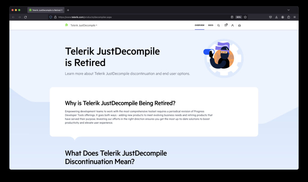
Behind the scene, the Java compiler will generate anonymous class that we can decompile and inspect closely. For the purpose of this post I am going to use fernflower decompiler. Here is the output for MyActivity$1 class.

package com.example;

import android.view.View;
import android.view.View.OnClickListener;
import android.widget.TextView;

class MyActivity$1 implements OnClickListener {
   // $FF: synthetic field
   final TextView val$txt;
   // $FF: synthetic field
   final MyActivity this$0;

   MyActivity$1(MyActivity this$0, TextView var2) {
      this.this$0 = this$0;
      this.val$txt = var2;
   }

   public void onClick(View view) {
      this.val$txt.setText("Count:" + MyActivity.access$004(this.this$0));
   }
}

We can see the Java compiler generates code that:
1) captures the variable txt
2) deals with ++count expression

This means that the click handler object holds references to the objects it accesses in its closure. We can call this class stateful as it has class members. Fairly trivial observation.

Let’s take a look again at the previous JavaScript code.

var button = new android.widget.Button(context);
button.setOnClickListener(new android.view.View.OnClickListener({
   onClick: function() {
      // do some work
   }
}));

We access the button widget and call its setOnClickListener method with some argument. This means that we should have instantiated Java object which implements OnClickListener so that the button can use it later. You can find the class implementation for that object in your project platform directory

[proj_dir]/platforms/android/src/main/java/com/tns/gen/android/view/View_OnClickListener.java

Let’s see what the actual implementation is.

package com.tns.gen.android.view;

public class View_OnClickListener
       implements android.view.View.OnClickListener {
  public View_OnClickListener() {
    com.tns.Runtime.initInstance(this);
  }

  public void onClick(android.view.View param_0)  {
    java.lang.Object[] args = new java.lang.Object[1];
    args[0] = param_0;
    com.tns.Runtime.callJSMethod(this, "onClick", void.class, args);
  }
}

As we can see this class acts as a proxy and doesn’t have fields. We can call this class stateless. We don’t store information that we can use to describe its closure if any.

So, we saw that Java compiler generates classes that keep track of their closures while NativeScript generates classes that don’t keep track of their closures. This is a simple implication due to the fact the JavaScript is a dynamic language and the information of lexical scope is not enough to provide full static analysis. The full information about JavaScript closures can be obtain at run time only.

The ovals diagram I used in my previous post visualize the missing object reference to the closed object. So, now we have an understanding what happens in NativeScript runtime for Android. The current NativeScript, at the time of writing version 3.3, provides mechanism to “compensate” for the missing object references. To put it simply, for each JavaScript closure accessible from Java we traverse all reachable Java objects in order to keep them alive until the closure becomes unreachable from Java. Well, while we were able to describe the current solution in a single sentence it doesn’t mean it doesn’t have drawbacks. This solution could be very slow if an object with large hierarchy, like global, is reachable from some closure. If this is the case, the implication is that we will traverse the whole V8 heap on each GC.

Back then in 2014, when we hit this issue for the first time, we discussed the option to customize part of the V8 garbage collector in order to provide faster heap traversing. The drawback is slower upgrade cycle for V8 which means that JavaScriptCore engine will provide more features at given point in time. For example, it is not easy to explain to the developers why they can use class syntax for iOS but not for Android.

Motivation: we wanted to keep V8 customization at minimum so we can achieve relatively feature parity by upgrading V8 engine as soon as possible.

So, now we know traversing V8 heap can be slow, what else? The current implementation is incomplete and case-by-case driven. This means that it is updated when there are important and common memory usage patterns. For example, currently we don’t traverse Map and Set objects.

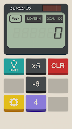
Let’s see what can happen in practice. Create a default app.

tns create app1

Run the app and make sure it works as expected.

Now, we have to go through the process of designing a user scenario where the runtime will crash. We know that the current implementation doesn’t traverse Map and Set objects. So, we have to make Java object which is reachable only through, let’s say, Map object. This is only the first part of our exercise. We also must take care to make it reachable through a closure. Finally, we must give a chance for GC to collect it before we use it. So, let’s code it.

function crash() {
    var m = new Map();
    m.set('o', new java.lang.Object() /* via the map only */);
    var h = new android.os.Handler(android.os.Looper.getMainLooper());
    h.post(new java.lang.Runnable({
        run: function() {
            console.log(m.get('o').hashCode());
        }
    }));
}

That’s all. Finally, we have to integrate crash within our application. We can do so by modifying onTap handler in [proj_dir]/app/main-view-model.js as follows:

viewModel.onTap = function() {
    crash();
    gc();
    java.lang.Runtime.getRuntime().gc();
    this.counter--;
    this.set("message", getMessage(this.counter));
}

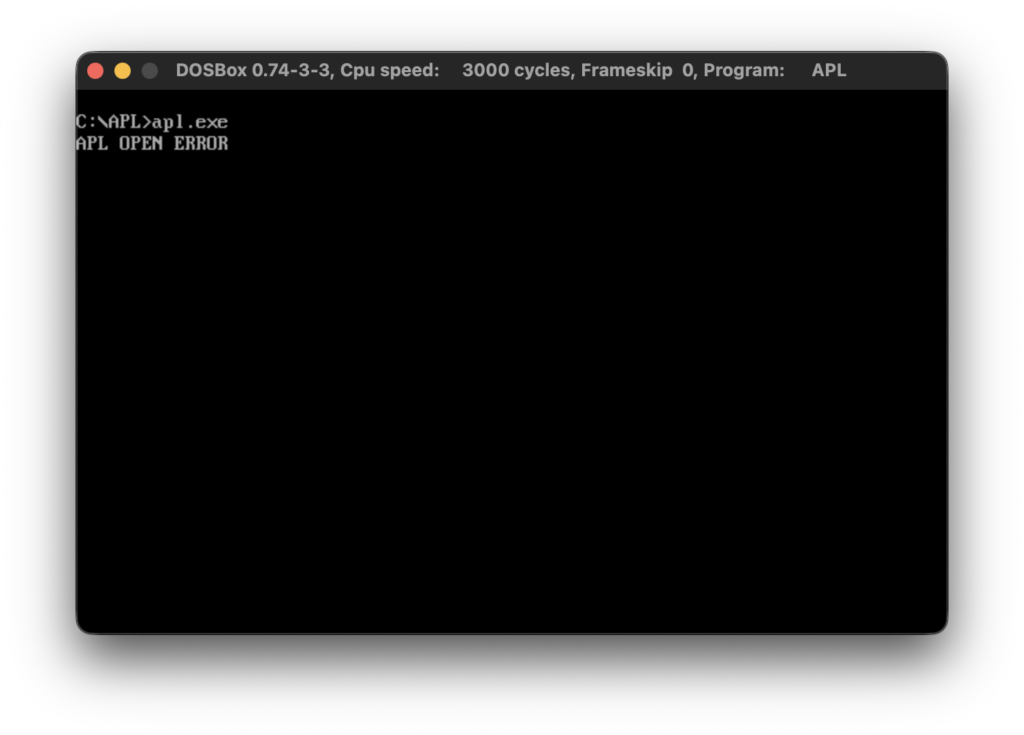
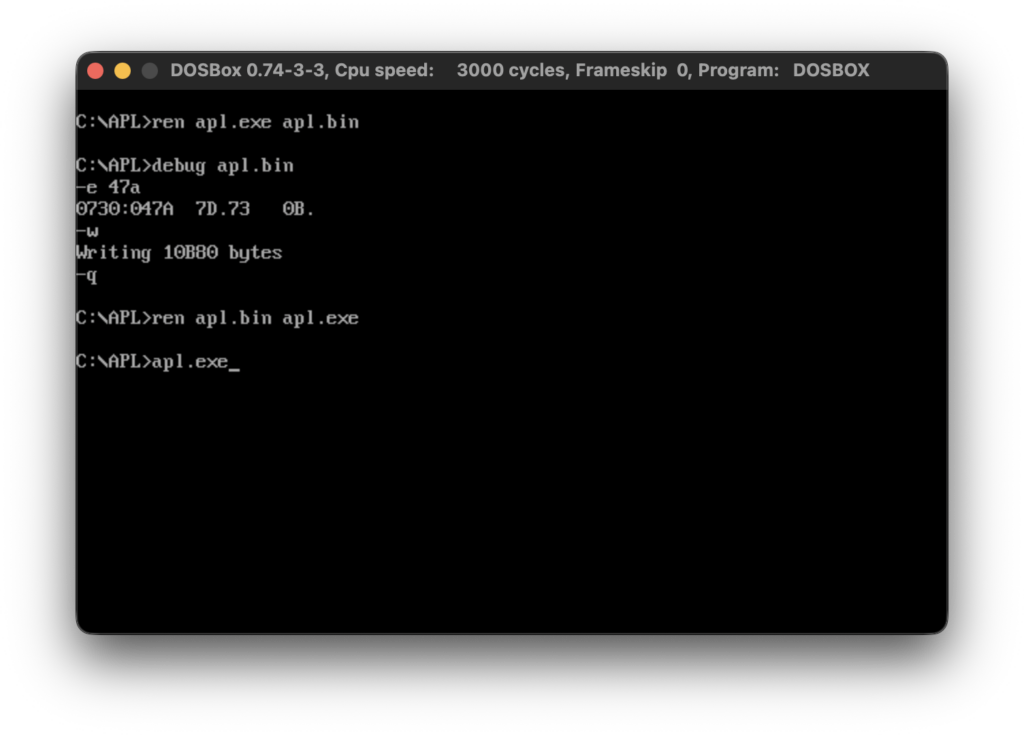
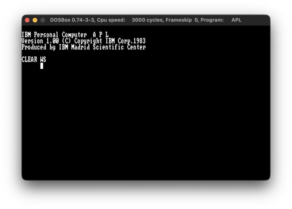
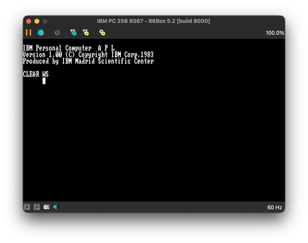
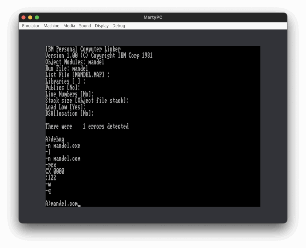
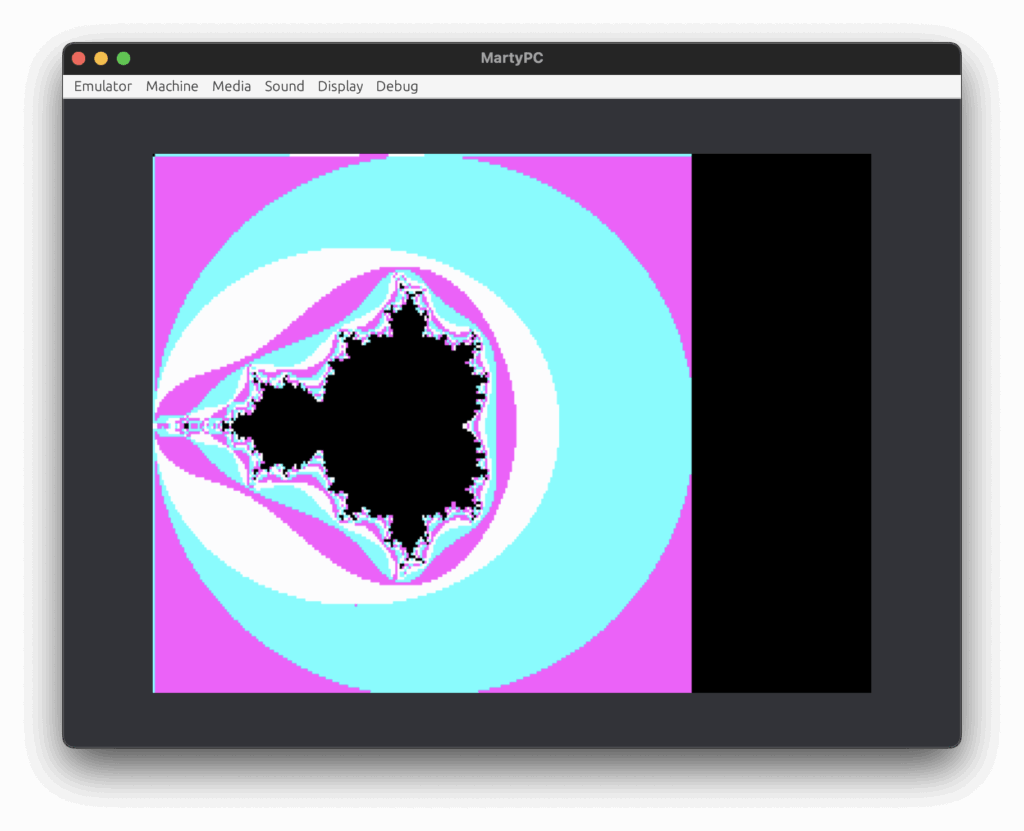
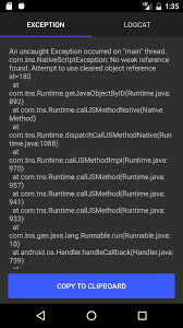
Run the app and click the button. You should get error screen similar to the following one.

Motivation: we wanted to evolve V8 heap traversing on case-by-case basis in order to traverse as little as possible.

Understanding this memory usage pattern (create object, set up object reachability, GC and usage) is a simple but powerful tool. With the current implementation the fix for Map and Set is similar to this one. Also, realizing that in the current implementation the missing references to the captured objects is the only reason for this error is critical for any further changes. This is well documented in the form of unit tests.

So far we discussed the drawbacks of the current implementation. Let’s say a few words about its advantages. First, and foremost, it keeps the current memory management model familiar to the existing Java and JavaScript developers. This is important in order to attract new developers. If two technologies, X and Y, solve similar problems and offer similar licenses, tools, etc., the developers are in favor for the one with simpler “mental model”. While introducing alloc/free or try/finally approach is powerful, it does not attract new developers because it sets higher entry level, less explicit approach. Another advantage, which is mostly for the platform developers, is the fact that current approach aligns well with many optimizations that can be applied. For example, taking advantage (introducing) of GC generations for the means of NativeScript runtime. Also, it allows per-application fine tuning of existing V8 flags (e.g, gc_intervalincremental_markingminor_mc, etc.). Tweaking V8 flags won’t have general impact when manual memory management is applied. In my opinion, tuning these flags is yet another way to help regular Joe shooting himself in the foot, but providing sane defaults and applying adaptive schemes very possible could be a huge win.

It is important to note that whatever approach is applied, this must be done carefully because of the risk of OOM exception. Introducing schemes like GC generation should consider the object memory weight. This will make obsolete the current approaches that use time and/or memory pressure heuristics. In general, such GC generation approach will pay off well.

I hope I shed more light on this challenging problem. Looking forward to see how the team is going to approach it. Good luck!

NativeScript release life cycle

I am glad to announce that yesterday we released NativeScript 2.4. This is all good, but in this post I would like to discuss the future. If you take a look at the next GitHub milestone you will see this

rc25

So, why 2.5.0-RC?

There are many reasons for this. Firstly, it is hard to make a feature right from the first time. And by “right” I don’t mean correct but also right from technical perspective. It’s not easy to say but every developer knows the difference a solution and the right solution. Secondly, often our requirements are incomplete and we need feedback as soon as possible in order to ship the right feature. Even with complete requirements it will take longer for development, thus delaying the user feedback. Following the analogy with minimum viable product (MVP), you can think of minimum viable technical implementation that (almost) meets the current requirements. As with many other release approaches it is a trade-off. Shipping RC is a sweet spot as we will offer reasonable product quality in a timely manner. Each RC will be followed shortly by an official release. So far, our release history shows that a week or two is enough to fix all corner-case issues and apply other minor fixes.

Of course, there are drawbacks. Probably the biggest one is that there will be increased operational costs for actual shipping RC or required changes in the test infrastructure for example. I think this is a good incentive to automate even more the existing processes and infrastructures so it will be a win-win situation. Stay tuned.